Automotive Brake Thermal Analysis

Objective:

Braking surfaces get heated due to frictional heating during braking. High temperature affects the braking performance and life of the braking system. This example demonstrates:

• Fluent setup and simulation using PyFluent

• Post processing using PyVista (3D Viewer) and Matplotlib (2D graphs)

Import required libraries/modules

import csv
from pathlib import Path

import ansys.fluent.core as pyfluent
from ansys.fluent.core import examples

PyVista

import ansys.fluent.visualization.pyvista as pv

Matplotlib

import matplotlib.pyplot as plt

Specifying save path

save_path can be specified as Path(“E:/”, “pyfluent-examples-tests”) or Path(“E:/pyfluent-examples-tests”) in a Windows machine for example, or Path(“~/pyfluent-examples-tests”) in Linux.

save_path = Path(pyfluent.EXAMPLES_PATH)

import_filename = examples.download_file(
    "brake.msh",
    "pyfluent/examples/Brake-Thermal-PyVista-Matplotlib",
    save_path=save_path,
)

Fluent Solution Setup

Launch Fluent session with solver mode

session = pyfluent.launch_fluent(
    mode="solver", show_gui=False, version="3ddp", precision="double", processor_count=2
)
session.check_health()

Import mesh

session.tui.file.read_case(import_filename)

Define models and material

session.tui.define.models.energy("yes", "no", "no", "no", "yes")
session.tui.define.models.unsteady_2nd_order_bounded("Yes")
session.tui.define.materials.copy("solid", "steel")

Solve only energy equation (conduction)

session.tui.solve.set.equations("flow", "no", "kw", "no")

Define disc rotation

(15.79 rps corresponds to 100 km/h car speed with 0.28 m of axis height from ground)

session.tui.define.boundary_conditions.set.solid(
    "disc1",
    "disc2",
    "()",
    "solid-motion?",
    "yes",
    "solid-omega",
    "no",
    -15.79,
    "solid-x-origin",
    "no",
    -0.035,
    "solid-y-origin",
    "no",
    -0.821,
    "solid-z-origin",
    "no",
    0.045,
    "solid-ai",
    "no",
    0,
    "solid-aj",
    "no",
    1,
    "solid-ak",
    "no",
    0,
    "q",
)

Apply frictional heating on pad-disc surfaces

Wall thickness 0f 2 mm has been assumed and 2e9 w/m3 is the heat generation which has been calculated from kinetic energy change due to braking.

session.tui.define.boundary_conditions.set.wall(
    "wall_pad-disc1",
    "wall-pad-disc2",
    "()",
    "wall-thickness",
    0.002,
    "q-dot",
    "no",
    2e9,
    "q",
)

Apply convection cooling on outer surfaces due to air flow

Outer surfaces are applied a constant htc of 100 W/(m2 K) and 300 K free stream temperature

session.tui.define.boundary_conditions.set.wall(
    "wall-disc*",
    "wall-geom*",
    "()",
    "thermal-bc",
    "yes",
    "convection",
    "convective-heat-transfer-coefficient",
    "no",
    100,
    "q",
)

Initialize

Initialize with 300 K temperature

session.tui.solve.initialize.initialize_flow()

Post processing setup

• Report definitions and monitor plots

• Set contour plot properties

• Set views and camera

• Set animation object

session.tui.solve.report_definitions.add(
    "max-pad-temperature",
    "volume-max",
    "field",
    "temperature",
    "zone-names",
    "geom-1-innerpad",
    "geom-1-outerpad",
)
session.tui.solve.report_definitions.add(
    "max-disc-temperature",
    "volume-max",
    "field",
    "temperature",
    "zone-names",
    "disc1",
    "disc2",
)

session.tui.solve.report_plots.add(
    "max-temperature",
    "report-defs",
    "max-pad-temperature",
    "max-disc-temperature",
    "()",
)

report_file_path = Path(save_path) / "max-temperature.out"
session.tui.solve.report_files.add(
    "max-temperature",
    "report-defs",
    "max-pad-temperature",
    "max-disc-temperature",
    "()",
    "file-name",
    str(report_file_path),
)


session.results.graphics.contour["contour-1"] = {
    "boundary_values": True,
    "color_map": {
        "color": "field-velocity",
        "font_automatic": True,
        "font_name": "Helvetica",
        "font_size": 0.032,
        "format": "%0.2e",
        "length": 0.54,
        "log_scale": False,
        "position": 1,
        "show_all": True,
        "size": 100,
        "user_skip": 9,
        "visible": True,
        "width": 6.0,
    },
    "coloring": {"smooth": False},
    "contour_lines": False,
    "display_state_name": "None",
    "draw_mesh": False,
    "field": "temperature",
    "filled": True,
    "mesh_object": "",
    "node_values": True,
    "range_option": {"auto_range_on": {"global_range": True}},
}


session.tui.display.objects.create(
    "contour",
    "temperature",
    "field",
    "temperature",
    "surface-list",
    "wall*",
    "()",
    "color-map",
    "format",
    "%0.1f",
    "q",
    "range-option",
    "auto-range-off",
    "minimum",
    300,
    "maximum",
    400,
    "q",
    "q",
)


session.tui.display.views.restore_view("top")
session.tui.display.views.camera.zoom_camera(2)
session.tui.display.views.save_view("animation-view")

session.tui.solve.animate.objects.create(
    "animate-temperature",
    "animate-on",
    "temperature",
    "frequency-of",
    "flow-time",
    "flow-time-frequency",
    0.05,
    "view",
    "animation-view",
    "q",
)

Run simulation

• Run simulation for 2 seconds flow time

• Set time step size

• Set number of time steps and maximum number of iterations per time step

session.tui.solve.set.transient_controls.time_step_size(0.01)
session.tui.solve.dual_time_iterate(200, 5)

Save simulation data

Write case and data files

save_case_data_as = Path(save_path) / "brake-final.cas.h5"
session.tui.file.write_case_data(save_case_data_as)

Post processing with PyVista (3D visualization)

Create a graphics session

graphics_session1 = pv.Graphics(session)

Temperature contour object

contour1 = graphics_session1.Contours["temperature"]

Check available options for contour object

contour1()

Set contour properties

contour1.field = "temperature"
contour1.surfaces_list = [
    "wall-disc1",
    "wall-disc2",
    "wall-pad-disc2",
    "wall_pad-disc1",
    "wall-geom-1-bp_inner",
    "wall-geom-1-bp_outer",
    "wall-geom-1-innerpad",
    "wall-geom-1-outerpad",
]
contour1.range.option = "auto-range-off"
contour1()
contour1.range.auto_range_off.minimum = 300
contour1.range.auto_range_off.maximum = 400

Display contour

contour1.display()

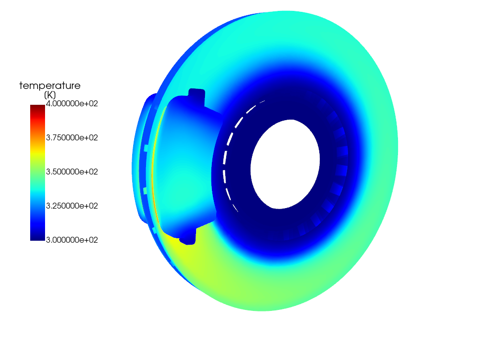
Brake Surface Temperature

Post processing with Matplotlib (2D graph)

Read monitor file

X = []
Y = []
Z = []
i = -1
with open(report_file_path, "r") as datafile:
    plotting = csv.reader(datafile, delimiter=" ")
    for rows in plotting:
        i = i + 1
        if i > 2:
            X.append(float(rows[3]))
            Y.append(float(rows[2]))
            Z.append(float(rows[1]))

Plot graph

plt.title("Maximum Temperature", fontdict={"color": "darkred", "size": 20})
plt.plot(X, Z, label="Max. Pad Temperature", color="red")
plt.plot(X, Y, label="Max. Disc Temperature", color="blue")
plt.xlabel("Time (sec)")
plt.ylabel("Max Temperature (K)")
plt.legend(loc="lower right", shadow=True, fontsize="x-large")

Show graph

plt.show()

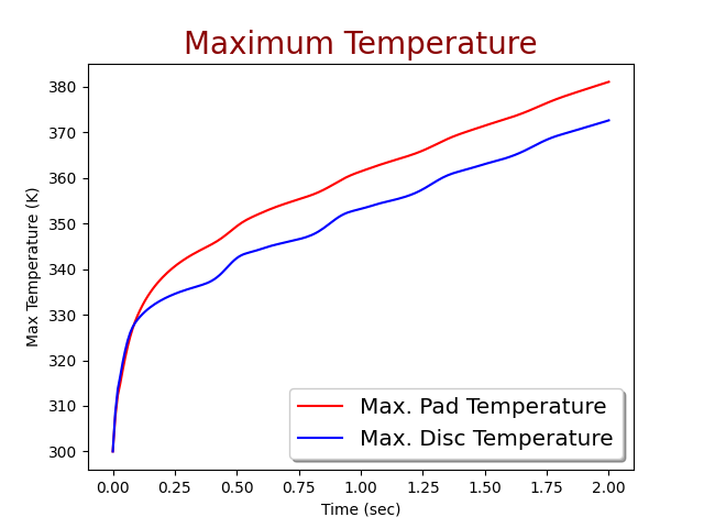
Brake Maximum Temperature

Close the session

session.exit()

# sphinx_gallery_thumbnail_path = '_static/brake_surface_temperature-thumbnail.png'