Tyler-Sofrin Compressor Modes Post-Processing

Objective

This example demonstrates PyFluent API’s for

• Read a case and data file

• Create monitor points to calculate Fourier coefficients

• Write Fourier coefficients to a file

• Tyler-Sofrin mode Plot using the matplotlib library

Background

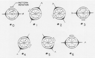
Tyler and Sofrin (1961) demonstrated that interactions between a rotor and a stator result in an infinite set of spinning modes. Each Tyler-Sofrin (TS) mode exhibits an m-lobed pattern and rotates at a speed given by the following equation:

\(\text{speed} = \frac{BnΩ}{m}\) Where:

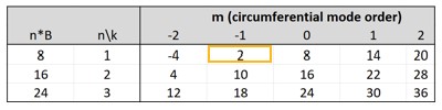
• m is the Tyler-Sofrin mode number, defined as ‘m = nB + kV’

• n is the impeller frequency harmonic

• k is the vane harmonic

• B is the number of rotating blades

• V is the number of stationary vanes

• Ω is the Rotor shaft speed, rad/s

Example:

• 8-blade rotor interacting with a 6-vane stator

• 2-lobed pattern turning at (8)(1)/(2) = 4 times shaft speed

Example Table

Tyler-Sofrin Modes

Example Note: Discrete Fourier Transform (DFT)

• In order to calculate the pressure related to each TS-mode, extend the simulation and perform the DFT of pressure at the desired blade passing frequency harmonics.

• Disable the Hanning windowing (specifically for periodic flows like this one) to avoid getting half the expected magnitudes for periodic flows. Make sure to set the windowing parameter to ‘None’ when specifying the Discrete Fourier Transform (DFT) in the graphical user interface (GUI).

• The DFT data will only be accurate if the sampling is done across the entire specified sampling period.

Note

The .cas/.dat file provided with this example is for demonstration purposes only. A finer mesh is necessary for accurate acoustic analysis. This example uses data sets generated with Ansys Fluent V2023R2.

Post-Processing Implementation

Import required libraries/modules

import math
from pathlib import Path
import random

import ansys.fluent.core as pyfluent
from ansys.fluent.core import examples
import matplotlib.pyplot as plt
import numpy as np

Specifying save path

save_path can be specified as:

• Path(“E:/”, “pyfluent-examples-tests”) or

• Path(“E:/pyfluent-examples-tests”) in a Windows machine for example, or

• Path(“~/pyfluent-examples-tests”) in Linux.

save_path = Path(pyfluent.EXAMPLES_PATH)

Downloading cas/dat file

import_filename = examples.download_file(
    "axial_comp_fullWheel_DFT_23R2.cas.h5",
    "pyfluent/examples/Tyler-Sofrin-Modes-Compressor",
)  # noqa: E501

examples.download_file(
    "axial_comp_fullWheel_DFT_23R2.dat.h5",
    "pyfluent/examples/Tyler-Sofrin-Modes-Compressor",
    save_path=save_path,
)

Launch Fluent session

session = pyfluent.launch_fluent(
    show_gui=True, processor_count=4, product_version="23.2.0"
)

Reading case and data file

Note

The dat file should correspond to the already completed DFT simulation.

session.tui.file.read_case_data(import_filename)

Define User constant/variables

Note

The variable names should match the ones written from the DFT and can be identified by manually examining the solution variables as shown below:

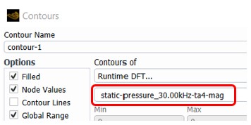
varname = [
    "mean-static-pressure-dataset",
    "dft-static-pressure_10.00kHz-ta",
    "dft-static-pressure-1_21.43kHz-ta",
    "dft-static-pressure-2_30.00kHz-ta",
]
n_mode = [0, 1, 2, 3]  # Impeller frequency harmonics
r = 0.082  # meters
z = -0.037  # meters
d_theta = 5  # degrees
m_max = 50  # maximum TS mode number

# Plot will be from -m_max to +m_max, incremented by m_inc
m_inc = 2  # TS mode increment

Create monitor points

for angle in range(0, 360, d_theta):
    x = math.cos(math.radians(angle)) * r
    y = math.sin(math.radians(angle)) * r
    session.tui.surface.point_surface("point-" + str(angle), x, y, z)

Compute Fourier coefficients at each monitor point (An, Bn)

An = np.zeros((len(varname), int(360 / d_theta)))
Bn = np.zeros((len(varname), int(360 / d_theta)))

for angle_ind, angle in enumerate(range(0, 360, d_theta)):
    for n_ind, variable in enumerate(varname):
        if len(variable) >= 4 and variable[:4] == "mean":
            session.solution.report_definitions.surface["mag-report"] = {
                "report_type": "surface-vertexavg",
                "surface_names": ["point-" + str(angle)],
                "field": str(variable),
            }
            mag = session.solution.report_definitions.compute(
                report_defs=["mag-report"]
            )
            mag = mag[0]["mag-report"][0]
            An[n_ind][angle_ind] = mag
            Bn[n_ind][angle_ind] = 0
        else:
            session.solution.report_definitions.surface["mag-report"] = {
                "report_type": "surface-vertexavg",
                "surface_names": ["point-" + str(angle)],
                "field": str(variable) + "-mag",
            }
            mag = session.solution.report_definitions.compute(
                report_defs=["mag-report"]
            )
            mag = mag[0]["mag-report"][0]
            session.solution.report_definitions.surface["phase-report"] = {
                "report_type": "surface-vertexavg",
                "surface_names": ["point-" + str(angle)],
                "field": str(variable) + "-phase",
            }
            phase = session.solution.report_definitions.compute(
                report_defs=["phase-report"]
            )
            phase = phase[0]["phase-report"][0]
            An[n_ind][angle_ind] = mag * math.cos(phase)
            Bn[n_ind][angle_ind] = -mag * math.sin(phase)

Write Fourier coefficients to file

Note

This step is only required if data is to be processed with other standalone tools. Update the path to the file accordingly.

fourier_coefficients_file = Path(save_path, "FourierCoefficients.txt")
with open(fourier_coefficients_file, "w") as f:
    f.write("n theta An Bn \n")

    for n_ind, variable in enumerate(varname):
        for ind, x in enumerate(An[n_ind, :]):
            f.write(
                str(n_mode[n_ind])
                + ","
                + str(ind * d_theta)
                + ","
                + str(An[n_ind, ind])
                + ","
                + str(Bn[n_ind, ind])
                + "\n"
            )

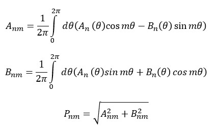
Calculate Resultant Pressure Field

Create list of m values based on m_max and m_inc

m_mode = range(-m_max, m_max + m_inc, m_inc)

# Initialize solution matrices with zeros
Anm = np.zeros((len(varname), len(m_mode)))
Bnm = np.zeros((len(varname), len(m_mode)))
Pnm = np.zeros((len(varname), len(m_mode)))

for n_ind, variable in enumerate(varname):  # loop over n modes
    for m_ind, m in enumerate(m_mode):  # loop over m modes
        for angle_ind, angle in enumerate(
            np.arange(0, math.radians(360), math.radians(d_theta))
        ):  # loop over all angles, in radians
            Anm[n_ind][m_ind] += An[n_ind][angle_ind] * math.cos(m * angle) - Bn[n_ind][
                angle_ind
            ] * math.sin(m * angle)
            Bnm[n_ind][m_ind] += An[n_ind][angle_ind] * math.sin(m * angle) + Bn[n_ind][
                angle_ind
            ] * math.cos(m * angle)
        Anm[n_ind][m_ind] = Anm[n_ind][m_ind] / (2 * math.pi) * math.radians(d_theta)
        Bnm[n_ind][m_ind] = Bnm[n_ind][m_ind] / (2 * math.pi) * math.radians(d_theta)
        Pnm[n_ind][m_ind] = math.sqrt(Anm[n_ind][m_ind] ** 2 + Bnm[n_ind][m_ind] ** 2)

# P_00 is generally orders of magnitude larger than that of other modes.
# Giving focus to other modes by setting P_00 equal to zero
Pnm[0][int(len(m_mode) / 2)] = 0

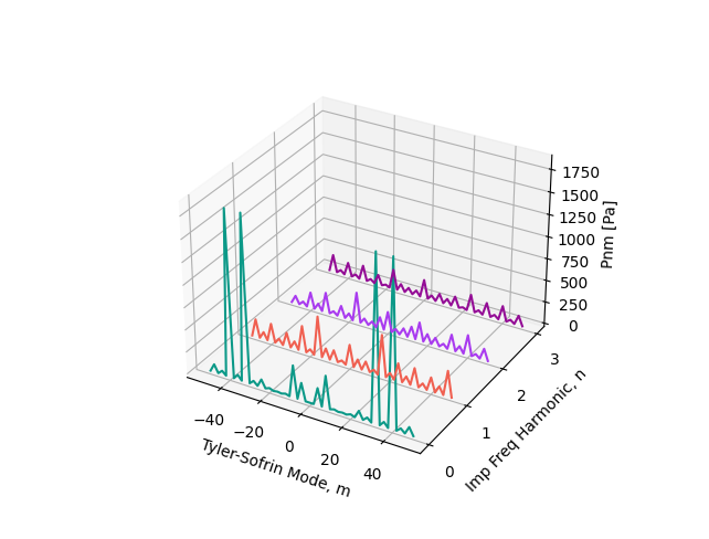
Plot Tyler-Sofrin modes

fig = plt.figure()
ax = plt.axes(projection="3d")
ax.set_xlabel("Tyler-Sofrin Mode, m")
ax.set_ylabel("Imp Freq Harmonic, n")
ax.set_zlabel("Pnm [Pa]")
plt.yticks(n_mode)
for n_ind, n in enumerate(n_mode):
    x = m_mode
    y = np.full(Pnm.shape[1], n)
    z = Pnm[n_ind]
    rgb = (random.random(), random.random(), random.random())
    ax.plot3D(x, y, z, c=rgb)
plt.show()

Tyler-Sofrin modes

Close the session

session.exit()

References

[1] J.M. Tyler and T. G. Sofrin, Axial Flow Compressor Noise Studies,1961 Manly Memorial Award.

# sphinx_gallery_thumbnail_path = '_static/ts_modes.png'