Note
Go to the end to download the full example code
Design of Experiments and Machine Learning model building#
Objective#
Water enters a Mixing Elbow from two Inlets; Hot (313 K) and Cold (293 K) and exits from Outlet. Using PyFluent in the background, this example runs Design of Experiments with Cold Inlet Velocity and Hot Inlet Velocity as Input Parameters and Outlet Temperature as an Output Parameter.
Results can be visualized using a Response Surface. Finally, Supervised Machine Learning Regression Task is performed to build the ML Model.
This example demonstrates:
Design of Experiment, Fluent setup and simulation using PyFluent.
Building of Supervised Machine Learning Model.
# sphinx_gallery_thumbnail_path = '_static/doe_ml_predictions_regression.png'
Import required libraries/modules#
from pathlib import Path

import ansys.fluent.core as pyfluent
from ansys.fluent.core import examples
import matplotlib.pyplot as plt
import numpy as np
import pandas as pd
import plotly.express as px
import plotly.graph_objects as go
import seaborn as sns
import tensorflow as tf
from tensorflow import keras
Specifying save path#
save_path can be specified as Path(“E:/”, “pyfluent-examples-tests”) or
Path(“E:/pyfluent-examples-tests”) in a Windows machine for example, or
Path(“~/pyfluent-examples-tests”) in Linux.
save_path = Path(pyfluent.EXAMPLES_PATH)

import_filename = examples.download_file(
    "elbow.cas.h5",
    "pyfluent/examples/DOE-ML-Mixing-Elbow",
    save_path=save_path,
)
Fluent Solution Setup#
Launch Fluent session with solver mode#
solver = pyfluent.launch_fluent(
    product_version="23.1.0",
    mode="solver",
    show_gui=False,
    version="3d",
    precision="double",
    processor_count=2,
)
solver.health_check_service.check_health()
Read case#
solver.tui.file.read_case(import_filename)
Design of Experiments#
Define Manual DOE as numpy arrays
Run cases in sequence
Populate results (Mass Weighted Average of Temperature at Outlet) in resArr
coldVelArr = np.array([0.1, 0.2, 0.3, 0.4, 0.5, 0.6, 0.7])
hotVelArr = np.array([0.8, 1, 1.2, 1.4, 1.6, 1.8, 2.0])
resArr = np.zeros((coldVelArr.shape[0], hotVelArr.shape[0]))

for idx1, coldVel in np.ndenumerate(coldVelArr):
    for idx2, hotVel in np.ndenumerate(hotVelArr):
        solver.setup.boundary_conditions.velocity_inlet["cold-inlet"].vmag = {
            "option": "value",
            "value": coldVel,
        }

        solver.setup.boundary_conditions.velocity_inlet["hot-inlet"].vmag = {
            "option": "value",
            "value": hotVel,
        }

        solver.tui.solve.initialize.initialize_flow("yes")
        solver.tui.solve.iterate(200)

        res_tui = solver.scheme_eval.exec(
            (
                "(ti-menu-load-string "
                '"/report/surface-integrals/mass-weighted-avg outlet () '
                'temperature no")',
            )
        )
        resArr[idx1][idx2] = eval(res_tui.split(" ")[-1])
Close the session#
solver.exit()
Plot Response Surface using Plotly#
fig = go.Figure(data=[go.Surface(z=resArr.T, x=coldVelArr, y=hotVelArr)])

fig.update_layout(
    title={
        "text": "Mixing Elbow Response Surface",
        "y": 0.9,
        "x": 0.5,
        "xanchor": "center",
        "yanchor": "top",
    }
)

fig.update_layout(
    scene=dict(
        xaxis_title="Cold Inlet Vel (m/s)",
        yaxis_title="Hot Inlet Vel (m/s)",
        zaxis_title="Outlet Temperature (K)",
    ),
    width=600,
    height=600,
    margin=dict(l=80, r=80, b=80, t=80),
)
fig.show()
Supervised ML for a Regression Task#
Create Pandas Dataframe for ML Model Input#
coldVelList = []
hotVelList = []
ResultList = []

for idx1, coldVel in np.ndenumerate(coldVelArr):
    for idx2, hotVel in np.ndenumerate(hotVelArr):
        coldVelList.append(coldVel)
        hotVelList.append(hotVel)
        ResultList.append(resArr[idx1][idx2])

tempDict = {"coldVel": coldVelList, "hotVel": hotVelList, "Result": ResultList}

df = pd.DataFrame.from_dict(tempDict)

from sklearn.compose import ColumnTransformer
from sklearn.model_selection import train_test_split
from sklearn.pipeline import Pipeline
from sklearn.preprocessing import PolynomialFeatures, StandardScaler
Using scikit-learn#
Prepare Features (X) and Label (y) using a Pre-Processing Pipeline
Train-Test (80-20) Split
Add Polynomial Features to improve ML Model
poly_features = PolynomialFeatures(degree=2, include_bias=False)

transformer1 = Pipeline(
    [
        ("poly_features", poly_features),
        ("std_scaler", StandardScaler()),
    ]
)


x_ct = ColumnTransformer(
    [
        ("transformer1", transformer1, ["coldVel", "hotVel"]),
    ],
    remainder="drop",
)

train_set, test_set = train_test_split(df, test_size=0.2, random_state=42)

X_train = x_ct.fit_transform(train_set)
X_test = x_ct.fit_transform(test_set)

y_train = train_set["Result"]
y_test = test_set["Result"]
y_train = np.ravel(y_train.T)
y_test = np.ravel(y_test.T)
Define functions for:
Cross-Validation and Display Scores (scikit-learn)
Training the Model (scikit-learn)
Prediction on Unseen/Test Data (scikit-learn)
Parity Plot (Matplotlib and Seaborn)
from pprint import pprint  # noqa: F401

from sklearn.ensemble import RandomForestRegressor  # noqa: F401
from sklearn.linear_model import LinearRegression  # noqa: F401
from sklearn.metrics import r2_score
from sklearn.model_selection import RepeatedKFold, cross_val_score
from xgboost import XGBRegressor

np.set_printoptions(precision=2)


def display_scores(scores):
    print("\nCross-Validation Scores:", scores)
    print("Mean:%0.2f" % (scores.mean()))
    print("Std. Dev.:%0.2f" % (scores.std()))


def fit_and_predict(model):
    cv = RepeatedKFold(n_splits=5, n_repeats=3, random_state=42)
    cv_scores = cross_val_score(
        model, X_train, y_train, scoring="neg_mean_squared_error", cv=cv
    )
    rmse_scores = np.sqrt(-cv_scores)
    display_scores(rmse_scores)

    model.fit(X_train, y_train)
    train_predictions = model.predict(X_train)
    test_predictions = model.predict(X_test)
    print(train_predictions.shape[0])
    print("\n\nCoefficient Of Determination")
    print("Train Data R2 Score: %0.3f" % (r2_score(train_predictions, y_train)))
    print("Test Data R2 Score: %0.3f" % (r2_score(test_predictions, y_test)))
    print(
        "\n\nPredictions - Ground Truth (Kelvin): ", (test_predictions - y_test), "\n"
    )
    #    print("\n\nModel Parameters:")
    #    pprint(model.get_params())

    com_train_set = train_set
    com_test_set = test_set

    train_list = []
    for i in range(train_predictions.shape[0]):
        train_list.append("Train")

    test_list = []
    for i in range(test_predictions.shape[0]):
        test_list.append("Test")

    com_train_set["Result"] = train_predictions.tolist()
    com_train_set["Set"] = train_list
    com_test_set["Result"] = test_predictions.tolist()
    com_test_set["Set"] = test_list

    df_combined = pd.concat([com_train_set, com_test_set])

    df_combined.to_csv("PyFluent_Output.csv", header=True, index=False)

    fig = plt.figure(figsize=(12, 5))

    fig.add_subplot(121)
    sns.regplot(x=y_train, y=train_predictions, color="g")
    plt.title("Train Data", fontsize=16)
    plt.xlabel("Ground Truth", fontsize=12)
    plt.ylabel("Predictions", fontsize=12)

    fig.add_subplot(122)
    sns.regplot(x=y_test, y=test_predictions, color="g")
    plt.title("Unseen Data", fontsize=16)
    plt.xlabel("Ground Truth", fontsize=12)
    plt.ylabel("Predictions", fontsize=12)

    plt.tight_layout()
    plt.show()
Select the Model from Linear, Random Forest or XGBoost#
Call fit_and_predict
# model = LinearRegression()
model = XGBRegressor(
    n_estimators=100, max_depth=10, eta=0.3, subsample=0.8, random_state=42
)
# model = RandomForestRegressor(random_state=42)

fit_and_predict(model)
Show graph#
plt.show()
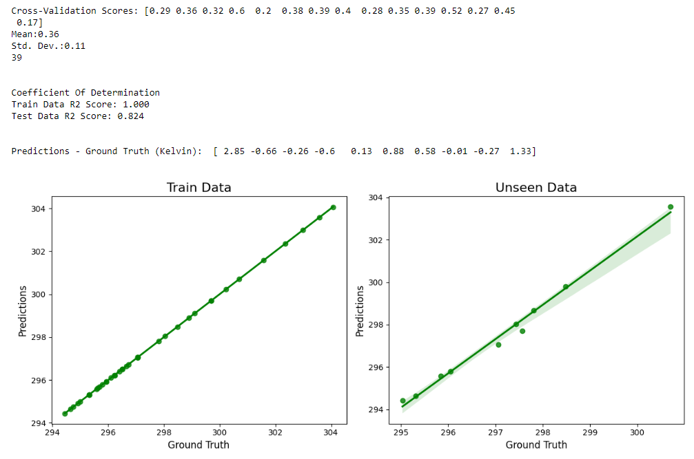
Regression Model Predictions
3D Visualization of Model Predictions on Train & Test Set#
df = pd.read_csv("PyFluent_Output.csv")

fig = px.scatter_3d(df, x="coldVel", y="hotVel", z="Result", color="Set")
fig.update_traces(marker=dict(size=4))
fig.update_layout(legend=dict(yanchor="top", y=1, xanchor="left", x=0.0))

fig.add_traces(go.Surface(z=resArr.T, x=coldVelArr, y=hotVelArr))

fig.update_layout(
    title={
        "text": "Mixing Elbow Response Surface",
        "y": 0.9,
        "x": 0.5,
        "xanchor": "center",
        "yanchor": "top",
    }
)

fig.update_layout(
    scene=dict(
        xaxis_title="Cold Inlet Vel (m/s)",
        yaxis_title="Hot Inlet Vel (m/s)",
        zaxis_title="Outlet Temperature (K)",
    ),
    width=500,
    height=500,
    margin=dict(l=80, r=80, b=80, t=80),
)

fig.show()
TensorFlow and Keras Neural Network Regression#
print("TensorFlow version is:", tf.__version__)
keras.backend.clear_session()
np.random.seed(42)
tf.random.set_seed(42)

model = keras.models.Sequential(
    [
        keras.layers.Dense(
            20,
            activation="relu",
            input_shape=X_train.shape[1:],
            kernel_initializer="lecun_normal",
        ),
        keras.layers.BatchNormalization(),
        keras.layers.Dense(20, activation="relu", kernel_initializer="lecun_normal"),
        keras.layers.BatchNormalization(),
        keras.layers.Dense(20, activation="relu", kernel_initializer="lecun_normal"),
        keras.layers.BatchNormalization(),
        keras.layers.Dense(1),
    ]
)

optimizer = tf.keras.optimizers.Adam(learning_rate=0.1, beta_1=0.9, beta_2=0.999)

model.compile(loss="mean_squared_error", optimizer=optimizer)
checkpoint_cb = keras.callbacks.ModelCheckpoint(
    "my_keras_model.h5", save_best_only=True
)
early_stopping_cb = keras.callbacks.EarlyStopping(
    patience=30, restore_best_weights=True
)

model.summary()

# keras.utils.plot_model(model, show_shapes=True,) # to_file='dot_img.png', )

history = model.fit(
    X_train,
    y_train,
    epochs=250,
    validation_split=0.2,
    callbacks=[checkpoint_cb, early_stopping_cb],
)
model = keras.models.load_model("my_keras_model.h5")

print(history.params)

pd.DataFrame(history.history).plot(figsize=(8, 5))
plt.grid(True)
plt.show()

train_predictions = model.predict(X_train)
test_predictions = model.predict(X_test)
train_predictions = np.ravel(train_predictions.T)
test_predictions = np.ravel(test_predictions.T)
print(test_predictions.shape)

print("\n\nTrain R2: %0.3f" % (r2_score(train_predictions, y_train)))
print("Test R2: %0.3f" % (r2_score(test_predictions, y_test)))
print("Predictions - Ground Truth (Kelvin): ", (test_predictions - y_test))

fig = plt.figure(figsize=(12, 5))

fig.add_subplot(121)
sns.regplot(x=y_train, y=train_predictions, color="g")
plt.title("Train Data", fontsize=16)
plt.xlabel("Ground Truth", fontsize=12)
plt.ylabel("Predictions", fontsize=12)

fig.add_subplot(122)
sns.regplot(x=y_test, y=test_predictions, color="g")
plt.title("Test/Unseen Data", fontsize=16)
plt.xlabel("Ground Truth", fontsize=12)
plt.ylabel("Predictions", fontsize=12)

plt.tight_layout()
Show graph#
plt.show()
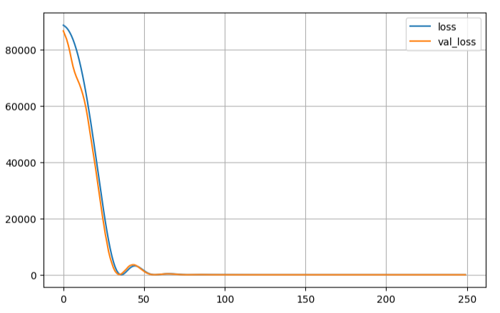
Neural Network Validation Loss
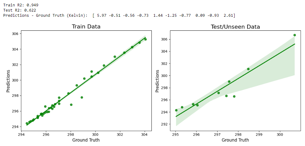
Neural Network Predictions
Total running time of the script: (0 minutes 0.000 seconds)